Analysing a Two-dimensional Pore Water Section using Dipole-Dipole Resistivity Methods
1 Aim
To analyse a two-dimensional vertical section of Earth and analyse the pore water content using dipole-dipole resistivity measurements.
2 Theory
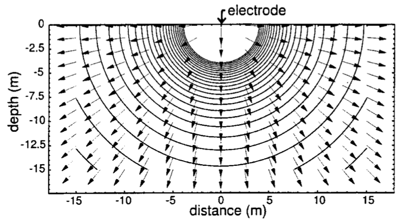
Consider an infinite and homogeneous Earth of resistivity \(\rho\). Let the voltage at infinity be \(U_\infty=0\), and let us apply a voltage at the origin as in figure 1. Ohm's law states \(V=IR\), where \(V\) is the potential drop through the soil. In terms of the resistivity, this means: $$V=I\frac{\rho l}{A}$$ where \(l\) is the distance from the voltage applied, and \(A\) is the surface area current travels through at distance \(l\). Note that here \(l=r\), the radial distance from the origin. This equation shows that the drop in voltage depends on the distance travelled through the Earth, i.e. equipotential surfaces will all be equidistant from the origin. Noting that \(A\) forms a hemisphere gives \(A=\frac{1}{2}4\pi r^2\), so:
\begin{equation} V(\mathbf{r})=I\frac{\rho}{2\pi r} \label{eq:V_from_node} \end{equation}|
Figure 1: Applied voltage on homogeneous Earth [herman2001introduction]. Arrows indicate conventional current flow, and lines indicate equipotential surfaces. |
Figure 2: Two applied voltages on homogeneous Earth [herman2001introduction]. |
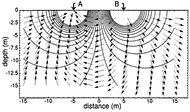
Extending this idea to incorporate two applied voltages can be accomplished through superposition. Figure 2 shows the equipotential surfaces and currents caused by two equal and opposite applied voltages. The corresponding extension to \eqref{eq:V_from_node} for two sources is:
\begin{align} V(\mathbf{r})&=I\frac{\rho}{2\pi\left|\mathbf{r}-\mathbf{r_a}\right|}-I\frac{\rho}{2\pi\left|\mathbf{r}-\mathbf{r_b}\right|} \notag\\ V(\mathbf{r})&=I\frac{\rho}{2\pi}\left[\frac{1}{\left|\mathbf{r}-\mathbf{r_a}\right|}-\frac{1}{\left|\mathbf{r}-\mathbf{r_b}\right|}\right] \label{eq:V_from_dipole} \end{align}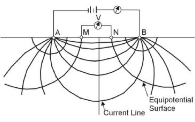
Figure 3: Applied current, and two voltage test points [1].
However, since \(V_\infty\) cannot be measured in a practical test, two separate voltage measurements must be made and the difference used in order to gain meaningful results. Such a measurement can be made with the experimental setup shown in figure 3. Using \eqref{eq:V_from_dipole} and assuming that current is injected from node \(A\) to node \(B\), the voltage between nodes \(M\) and \(N\) is given by:
\begin{align} V_{MN}=V(M)-V(N)&=I\frac{\rho}{2\pi}\left[\frac{1}{\left|\mathbf{r_m}-\mathbf{r_a}\right|}-\frac{1}{\left|\mathbf{r_m}-\mathbf{r_b}\right|}-\frac{1}{\left|\mathbf{r_n}-\mathbf{r_a}\right|}+\frac{1}{\left|\mathbf{r_n}-\mathbf{r_b}\right|}\right] \label{eq:geom_K}\\ &=I\frac{\rho}{2\pi}\frac{1}{K} \label{eq:V_homo} \end{align}where \(K\) is known as the geometric factor, dependent on the electrode setup.
Where the Earth in no longer homogeneous, \(\rho\) may be constantly varying, thus a given electrode setup can only measure a weighted indication of the local resistivity. Therefore, once a heterogeneous Earth is considered, we refer to the measured resistivity as the apparent resistivity, \(\rho_a\) [1]. Rearranging \eqref{eq:V_homo}
\begin{equation} \rho_a=2\pi K \frac{V}{I} \label{eq:apparent_resistivity} \end{equation}2.1 Dipole-dipole array
|
Figure 4: Dipole-dipole setup [1]. |
Figure 5: Electrode labelling. |
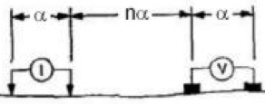
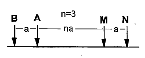
A dipole-dipole array uses separated dipoles for each pair, the current injectors and the voltage measuring. This setup is depicted in figures 4 and 5. Let the left and right current nodes be nodes \(b\) and \(a\) respectively, and the left and right voltage nodes be \(m\) and \(n\) respectively. It can be seen that:
\begin{align} \left|\mathbf{r_m}-\mathbf{r_b}\right|&=(n+1)\alpha, & \left|\mathbf{r_n}-\mathbf{r_b}\right|&=(n+2)\alpha, \\ \left|\mathbf{r_m}-\mathbf{r_a}\right|&=n\alpha, & \left|\mathbf{r_n}-\mathbf{r_a}\right|&=(n+1)\alpha \end{align}Using the geometric factor definition from \eqref{eq:geom_K}, the geometric factor is given by:
\begin{align} \frac{1}{K}&=\left[\frac{1}{n\alpha}-\frac{1}{(n+1)\alpha}-\frac{1}{(n+1)\alpha}+\frac{1}{(n+2)\alpha}\right] \notag\\ \frac{1}{K}&=\left[\frac{1}{n\alpha}-\frac{2}{(n+1)\alpha}+\frac{1}{(n+2)\alpha}\right] \notag\\ \frac{1}{K}&=\frac{(n+1)(n+2)\alpha^2 - 2n(n+2)\alpha^2 + n(n+1)\alpha^2}{n(n+1)(n+2)\alpha^3} \notag\\ \frac{1}{K}&=\frac{1}{\alpha}\frac{2}{n(n+1)(n+2)} \notag\\ K&=\frac{1}{2}\alpha n(n+1)(n+2) \label{eq:K} \end{align}Combining \eqref{eq:apparent_resistivity} and \eqref{eq:K} gives the following [1]:
\begin{equation} \rho_a=\pi\alpha n(n+1)(n+2)\frac{V}{I} \label{eq:dipole} \end{equation}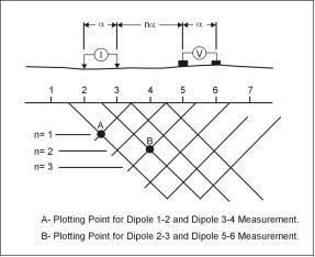
Figure 6: Varying \(n\) with a dipole-dipole array allows different depths to be explored [1].
Figure 6 demonstrates how using \eqref{eq:dipole}, and varying \(n\) allows a two-dimensional depth-resistivity profile to be produced. Since most soils have a relatively high resistivity, with the exception of metal ore deposits, most of the resistivity actually measured is due to the pore water content of the soil [1].
3 Materials
- the MiniStingTM earth resistivity meter
- the SwiftTM automatic electrode system
- associated cabling
- a 12 V DC battery
- two 12 node electrode cables
- 28 electrode stakes
- 28 alligator clips
- approximately 50 L of salted water
- a sledge hammer
- a laptop PC
- a GPS device (mobile phone)
4 Methodology
- The electrode stakes were spaced at 2.5 m intervals along a straight line, the intended measurement region, and were driven each 10 to 20 cm deep. Salt water was poured over each stake to ensure a good electrical connection with the earth.
- The two electrode cables were laid out end-to-end, alongside the electrodes. Each electrode stake was connected to the cable electrode using the alligator clips.
- A GPS device was used to measure the coordinates at the start, join, and end of the two electrode cables.
- The MiniSting, Swift, switch box, battery and electrode cabling
were connected as depicted in 7.
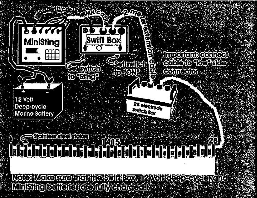
Figure 7: Hardware setup [advancedgeosciences2003].
- The MiniStingTM was configured with the parameters outlined in
1.
Table 1: MiniStingTM Parameters Parameter Setting Current 100 mA Max. Cycles 2 Accuracy 5% Measurement Time 1.2 s Voltage 200 V - A contact resistance test was run to ensure that an adequately low contact resistance was achieved.
- The MiniStingTM automatic dipole-dipole profile test was initiated.
- After measurement number 217, the current was increased to 150 mA as some measurements were failing and being recalculated, slowing the measurement process.
- After completion of the test, the results were uploaded to the PC and analysed with the AGI EarthImager 2D Inversion software [2].
- A second group also repeated a similar process, with a 3 m spacing. These results, labelled group 2, were also included for analysis.
5 Results
5.1 Group 1
Following are the results from group 1. Table 2 shows the GPS location measured along the cable. Figure 8 shows an approximate sketch of the setup also. Finally, the measured results are shown in figure 9.
| S 19 19' 46.4982” | E 146 45' 23.4786” |
| S 19 19' 46.5024” | E 146 45' 23.4786” |
| S 19 19' 46.5060” | E 146 45' 23.4900” |
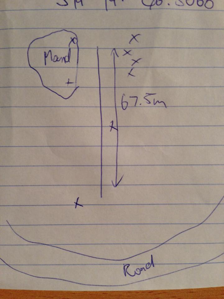
Figure 8: Sketch of approximate location. 'X's indicate trees.
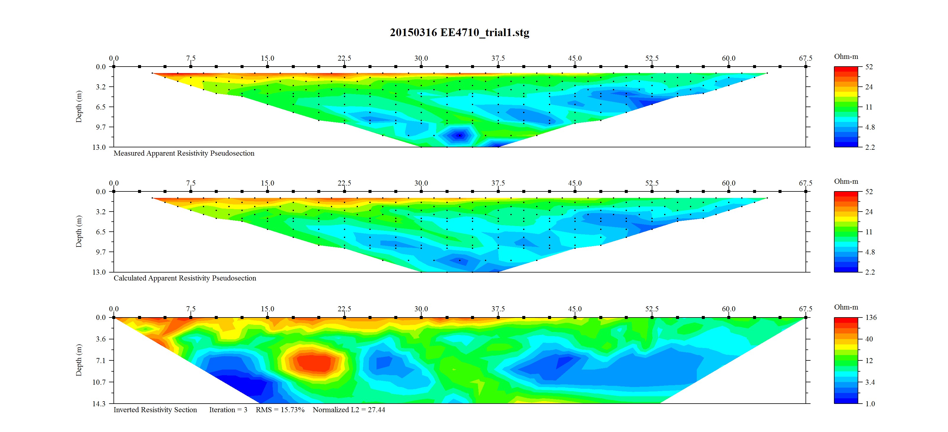
Figure 9: Group 1 Top) measured apparent resistivity, Bottom) calculated resistivity.
5.1.1 Observations
- Whilst inserting the electrodes that the more southern electrodes were more difficult to insert due to dryer and rockier ground.
- Measurements were made in May, as Townsville is coming out of the wet season. Last rainfall was in the order of weeks before.
5.2 Group 2
Following are the results from group 2, taken separately and for comparison. Table tbl:gps_2 shows the GPS location measured along the cable. The measured results are shown in 10.
| S 19 19' 57.38” | E 146 45' 25.70” |
| S 19 19' 56.50” | E 146 45' 25.91” |
| S 19 19' 55.83” | E 146 45' 26.17” |
| S 19 19' 55.02” | E 146 45' 26.52” |
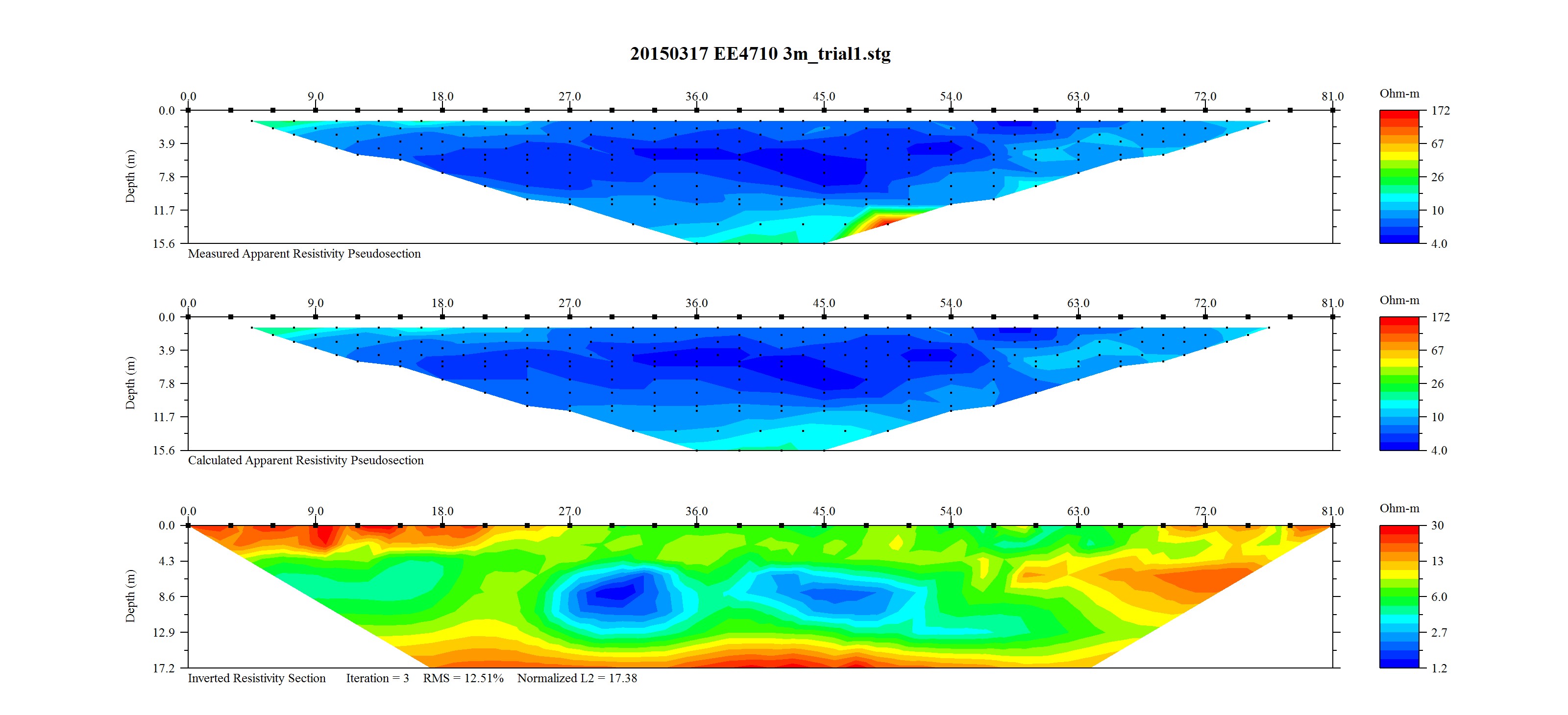
Figure 10: Group 2 Top) measured apparent resistivity, Bottom) calculated resistivity.
It was also noted by a supervisor of both groups that both groups laid node 1 as the south-most node, and that group 1's node 28 and group 2's node 24 were located at approximately the same location.
6 Analysis
Each group's GPS coordinates were plotted in order to compare the physical locations measured in each session. The results are shown in figure 11. However, the locations for group 1 were seen to be inaccurate, showing a location approximately 1 km north of the actual location. Therefore, sketched information from figure 8 was used for the group 1 location. An updated map is given in figure 12.
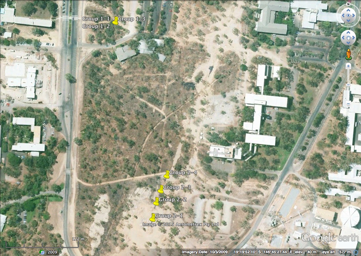
Figure 11: Measured GPS locations
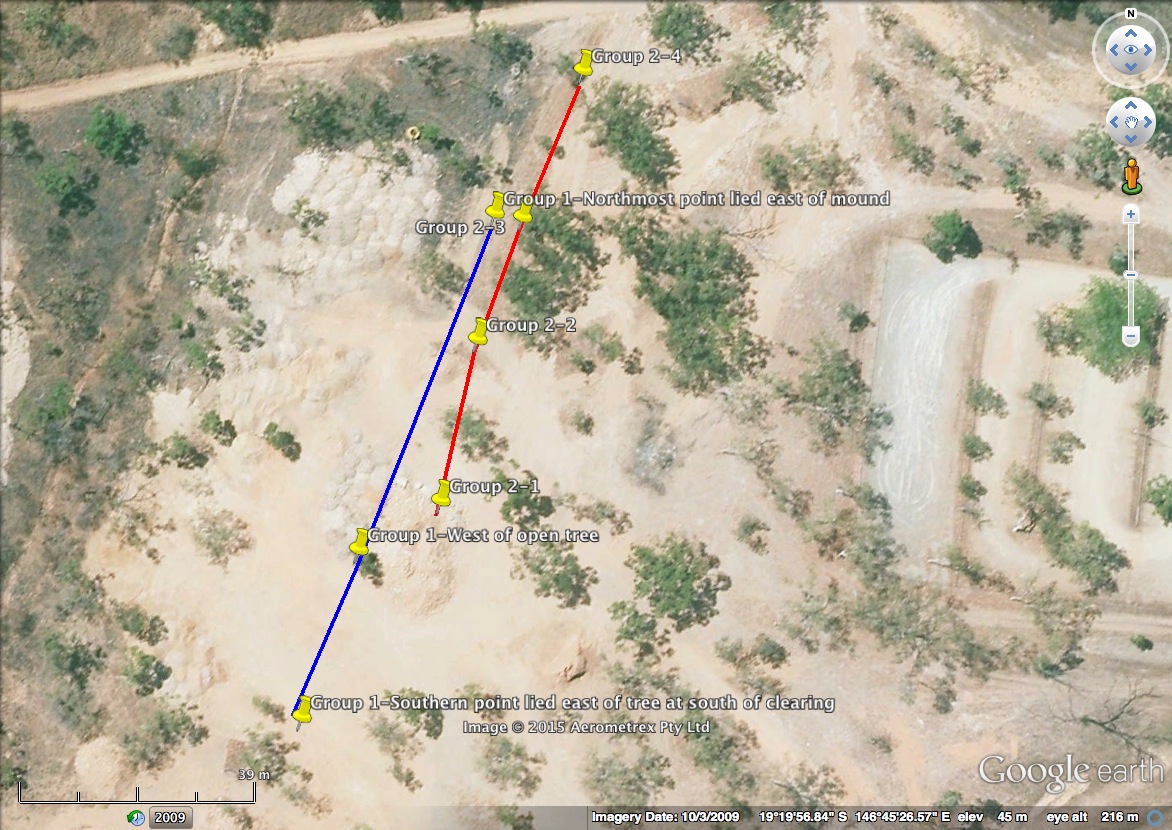
Figure 12: Estimated GPS locations, blue indicates group 1 and red indicates group 2.
The information in figures 9 and 10 both agreed with one-another and agreed with observations made at the site. It should be noted that the left side of the plots corresponded to the southern-most measurements. Both plots indicated a high surface resistance on the southern end of the line. Additionally, results in figure 9 Bottom) displayed a longer section of high surface resistance compared with those in figure 9 Bottom). This was consistent with the fact that group 1's cable ran further south. This was also consistent with observations that the more southern stakes were harder to insert. Harder and rockier soil is generally drier and less conductive, as it holds less pore water.
Both figures 9 and 10 showed two areas of lower resistivity at a depth of approximately 8–10 m. These sections also appeared to line up between the two results. This is better demonstrated in figure 13, where the results were scaled such that the group 1 size to group 2 size ratio was 2.5:3. Additionally, the two have been positioned such that group 1 node 28 aligns with group 2 node 24, as noted by the practical supervisor.
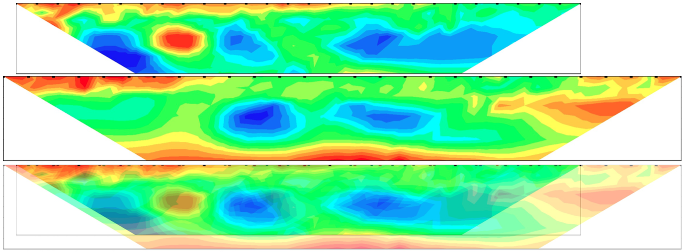
Figure 13: Top) Group 1 calculated resistivity scaled and positioned. Middle) Group 2 calculated resistivity scaled and positioned. Bottom) Group 1 and 2 calculated resistivity scaled and positioned.
Results in figure 13 supported one another, indicating accuracy in the measurements. Many of the common features physically aligned between the two images in figure 13, including:
- three regions of lower resistivity at approximately 8–10 m depth, although the south-most region was more apparent in group 1's results;
- a region of higher resistivity between the first two lower resistivity regions, which was again more apparent in group 1's results; and
- A shallow, high resistivity region along the southern surface.
Examination of figures 13 and 12 indicated that the latter mentioned region of high surface resistivity corresponded to an area with little tree coverage. Areas with fauna coverage however indicated a relatively high surface resistance. This was likely no coincidence, instead indicating that the lack of tree coverage had allowed the Sun to dry the surface in this area.
Figures 13 and 12 also showed that the two dominant regions of lower resistivity lied near the mound to the west of the measurements. It is possible that pore water in the mound remaining from the wet season had seeped down, leaving the measured region wetter than it would have otherwise been. This was also the region with the most tree coverage, which likely aided in pore water retention.
Continued examination of 13 showed the southern surface region of group 1's results displayed an odd pattern not seen in group 2's results, where underneath node 2 there was a low resistivity region. It is possible that this was indicative of a bad measurement. This may have also affected deeper regions, since an iterative estimation is used to correct for heterogeneities in the soil. This was supported by the two exaggerated regions of very high and very low resistivity measured deeper below this area in group 1 results. Therefore it is likely that the southern measurements of group 2 were more accurate than the southern measurements of group 1, and that these regions were not in actuality so exaggerated. It is possible these inconsistencies in group 1's measurements were due to the change in current from 100 mA to 150 mA halfway through the test.
7 Conclusion
The aim of the practical, to analyse a two-dimensional vertical section of Earth and analyse the pore water content using dipole-dipole resistivity measurements, was achieved. The results indicated a high surface resistivity over exposed areas of earth, and a relatively lower surface resistivity over regions shaded by trees. The analysis also showed evidence of pore water at a depth of approximately 8–10 m to the east of a nearby mound. It was determined to be likely this pore water seeped from the mound from the wet season, and was preserved by the shade of surrounding fauna.
An interesting additional conclusion was errors in the southern measurements of group 1's results, which propagated to show inconsistencies along the entire southern region. These errors were attributed to a change in supplied current halfway through the test.
References
| [1] | W. Wightman, F. Jalinoos, P. Sirles, and K. Hanna, “Application of geophysical methods to highway related problems,” 2004. |
| [2] | A. G. Inc., “EarthImager 2D.” https://www.agiusa.com/agi2dimg.shtml, 1999--2011. |