Finite Difference Method for a Numerical Solution to the Laplace Equation
1 Aim
To develop a numerical solution using to the the voltage and electrical field in a two-dimensional cross section of a coaxial cable of a given shape.
2 Theory
A numerical solution to a problem works by solving the problem over a series of discrete points rather than solving over the entire continuous domain. For a two-dimensional problem, this generally means solving over a grid. The grid must contain within it the entire problem domain, in this practical this means that the coaxial cable cross-section must be fully contained within the grid.
Additionally, the numerical solution is calculated iteratively. This means that a new estimate is made for each point based on the current estimates, and this is continuously updated. If the estimation method is accurate, the points will eventually converge towards the correct solution.
Voltage can be related to electric field, \(\textbf{E}\), in two dimensions by the following formulae:
\begin{align} \mathbf{E} &= -\nabla V \label{eq:V_E} \\ \mathbf{E} &= -\frac{\partial^2}{\partial x^2}V\mathbf{\hat{x}} - \frac{\partial^2}{\partial y^2}V\mathbf{\hat{y}} \label{eq:V_E_cart} \end{align}Combining \eqref{eq:V_E} with the property of the electric field that its divergence is 0, \(\nabla\cdot\mathbf{E}=0\) [5], yields Laplace's equation:
$$\nabla^2V=0$$
where \(\nabla^2\) is the Laplacian operator [1]. Laplace's equation is a partial differential equation, and can also be given for two dimensions in Cartesian form as:
\begin{equation} \frac{\partial^2 V}{\partial x^2}+\frac{\partial^2 V}{\partial y^2}=0 \label{eq:Laplace} \end{equation}Finding a solution to Laplace's equation required knowledge of the boundary conditions, and as such it is referred to as a boundary value problem (BVP). BVPs can be solved numerically using a method known as the finide difference (FD) method [2][3].
2.1 Finite Difference Method
In the FD method, differential equations are replace by their FD approximation. This approximation can be derived using the Taylor's theorem [2], given by:
\begin{equation} f(z)=\sum_{k=0}^{\infty}\frac{f^{(k)}(z_0)}{k!}(z-z_0)^k \label{eq:TS} \end{equation}where \(f\) is a function we are trying to solve for at point \(z\), given a known value \(f(z_0)\), and \(f^{(k)}\) is the \(k^{\text{th}}\) derivative of \(f\) [4]. A suitable grid for calculation of a coaxial cable cross-section is given in figure 1 Left}, and in figure 1 Right} is a close-up of the computational grid, used for approximation of \(\frac{\partial^n V}{\partial x^n}\) and \(\frac{\partial^n V}{\partial y^n}\).
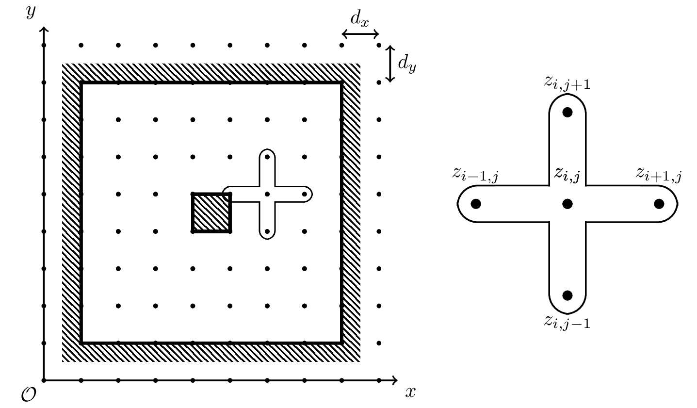
Figure 1: Left) A computational grid set up for a cross-section of a coaxial cable, in this case with a square shield and core. Right) A close up of the current point, \(V(i,j)\) and its neighbours. Here, \(i\), and \(j\) represent the \(x\) and \(y\) coordinated of the currently considered point respectively [3].
We will first consider a FD method for approximating the first derivative, followed by a method for the second derivative. Approximation by Taylor series (TS), as given in \eqref{eq:TS}, can be achieved by truncating the infinite sum. Truncating to three terms gives:
\begin{align} f(z) &= f(z_0) + f'(z_0)(z-z_0) + \frac{f''(z_0)}{2}(z-z_0)^2 + O((z-z_0)^3) \notag\\ f(z) &\approx f(z_0) + f'(z_0)(z-z_0) + \frac{f''(z_0)}{2}(z-z_0)^2 \label{eq:TS_approx} \end{align}If we consider \(z_0\) in \eqref{eq:TS_approx} to be a point on a one-dimensional computational grid, \(z_i\), and \(z\) to be the point to the left of \(z_i\), \(z_{i-1}=z_i-d_x\), this becomes:
\begin{equation} f(z_{i-1}) \approx f(z_i) - f'(z_i)(d_x) + \frac{f''(z_i)}{2}d_x^2 \label{eq:TS_approx_l} \end{equation}Similarly, if \(z_0=z_i\), and \(z\) is the point to the right of \(z_i\), \(z_{i+1}=z_i+d_x\), this becomes:
\begin{equation} f(z_{i+1}) \approx f(z_i) + f'(z_i)(d_x) + \frac{f''(z_i)}{2}d_x^2 \label{eq:TS_approx_r} \end{equation}Subtracting, \eqref{eq:TS_approx_r} \(-\) \eqref{eq:TS_approx_l} gives: $$f'(z_i) \approx \frac{f(z_{i+1}) - f(z_{i-1})}{2d_x}$$ which is known as the central difference approximation to the derivative [2]. Equations \eqref{eq:TS_approx_r} and \eqref{eq:TS_approx_l} can also be used to generate a second order derivative approximation. Summing, \eqref{eq:TS_approx_l} \(+\) \eqref{eq:TS_approx_r} gives [2]: $$f''(z_i) \approx \frac{f(z_{i-1}) - 2f(z_i) + f(z_{i+1})}{d_x^2}$$ Finally, a trivial extension into two dimensions yields:
\begin{align} \frac{\partial f}{\partial x} &\approx \frac{f(z_{i+1,j}) - f(z_{i-1,j})}{2d_x} \label{eq:1stO_FD_x} \\ \frac{\partial f}{\partial y} &\approx \frac{f(z_{i,j+1}) - f(z_{i,j-1})}{2d_y} \label{eq:1stO_FD_y} \\ \frac{\partial^2 f}{\partial x^2} &\approx \frac{f(z_{i-1,j}) - 2f(z_{i,j}) + f(z_{i+1,j})}{d_x^2} \label{eq:2ndO_FD_x} \\ \frac{\partial^2 f}{\partial y^2} &\approx \frac{f(z_{i,j-1}) - 2f(z_{i,j}) + f(z_{i,j+1})}{d_y^2} \label{eq:2ndO_FD_y} \end{align}The error associated with \eqref{eq:1stO_FD_x}, \eqref{eq:1stO_FD_y}, \eqref{eq:2ndO_FD_x}, and \eqref{eq:2ndO_FD_y} is \(O(\frac{d^3}{d})=O(d^2)\).
2.2 Solving Laplace's Equation for Voltage and Electric Field
Substituting \eqref{eq:2ndO_FD_x} and \eqref{eq:2ndO_FD_y} into \eqref{eq:Laplace} gives the discretised from of Laplace's equation:
$$\frac{V(z_{i-1,j}) - 2V(z_{i,j}) + V(z_{i+1,j})}{d_x^2} + \frac{V(z_{i,j-1}) - 2V(z_{i,j}) + V(z_{i,j+1})}{d_y^2} \approx 0 \notag\\$$
\begin{equation} V(z_{i,j}) \approx \frac{d_x^2(V(z_{i,j-1}) + V(z_{i,j+1})) + d_y^2 (V(z_{i-1,j}) + V(z_{i+1,j}))}{2(d_x^2 + d_y^2)} \label{eq:laplace_FD} \end{equation}If \(d_x=d_y\), this becomes [3]: $$V(z_{i,j}) \approx \frac{V(z_{i,j+1}) + V(z_{i-1,j}) + V(z_{i+1,j}) + V(z_{i,j-1})}{4}$$ which satisfies the condition of a solution to Laplace's equation that a point at the centre of an n-sphere should be the mean of its edges [1]. However, the form given in \eqref{eq:laplace_FD} will be used in this simulation to allow for independent \(x\) and \(y\) grid spacings.
Finite differences can also be used to calculate the electric field from the voltage. Substituting \eqref{eq:1stO_FD_x} and \eqref{eq:1stO_FD_y} into \eqref{eq:V_E_cart} gives:
\begin{equation} \mathbf{E} \approx -\frac{V(z_{i+1,j}) - V(z_{i-1,j})}{2d_x}\mathbf{\hat{x}} - \frac{V(z_{i,j+1}) - V(z_{i,j-1})}{2d_y}\mathbf{\hat{y}} \label{eq:E_V_FD} \end{equation}3 Methodology
- Using equations \eqref{eq:laplace_FD} and \eqref{eq:E_V_FD}, the
MATLAB code give in the appendix was developed. The following
describes each code block:
% Input Parametersshieldxs [...]: Shield polygon x coordinates.shieldys [...]: Shield polygon y coordinates.shieldv: Shield voltage.corexs [...]: Core polygon x coordinates.coreys [...]: Core polygon y coordinates.corev: Core voltage.gridsize [x,y]: No. x and y grid points.maxits: Maximum no. of iterations to perform.err: Maximum allowable error before convergence.
% Field (real units)The field is initialised to cover the coaxial cable cross section.
% Grid (pixels)A computational grid is defined over the field.
% Set grid initial valueInitialise outer shield voltages to shieldv, inner core voltages to corev, and space voltages to \(\frac{1}{2}(\texttt{shieldv}+\texttt{corev})\)
% iterationsIterate [eq:laplaceFD] for all points except edge points, reset core and shield voltages to initial values, and check for convergence.
% Calculate EUsing \eqref{eq:E_V_FD}, calculate the electric field. Also, ensure that the field inside the conductors is 0, preventing slight errors creeping in at the edges.
% Plot V and EPlot the resultant voltage and electric fields.
- The above simulation was run for a number of different cases. In
each, the outer shield was an equilateral triangle with sides of 10
cm, and the core was a square with sides of 2 cm, gridsize was
\(129\times129\), maxits was 10,000 and err was 0.01. Other test
parameters used are given in table 1.
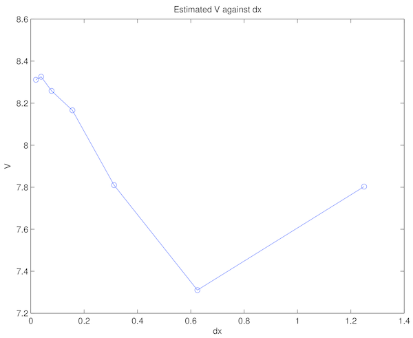
Table 1: Test Parameters Test no. shieldv corev 1 0 V 20 V 2 20 V 0 V 3 -10 V 10 V 4 10 V -10 V - In addition, the simulation was run using test conditions from test no. 1 for a range of grid sizes, \([2^n+1, 2^n+1]\) for \(n=3, 4, ..., 10\). Increasing the grid size allowed for smaller \(d_x\) and \(d_y\) values to be investigated, and their associated error.
4 Results
Results to the four experiments outlined in 1 are given in tables 2, 3, 4, and 5.
 |
 |
 |
 |
 |
 |
 |
 |
 |
5 Discussion
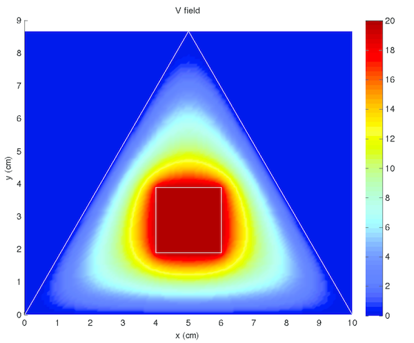
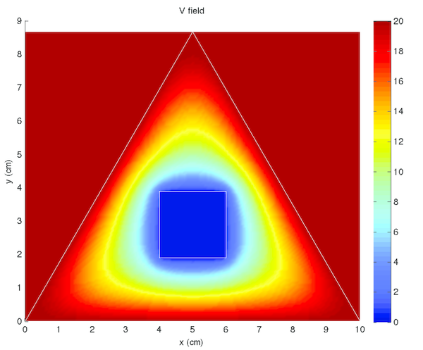
The simulations appeared to be accurate and results were logical and consistent with known properties of the voltage and electric field.
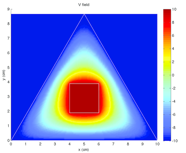
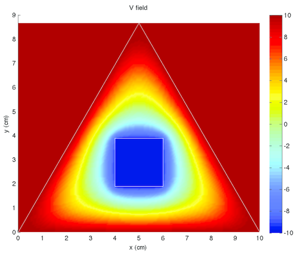
Voltage was constant within the conductors, both the shield and core, in tables 2, 3, 4, and 5 left) (although this was expected, as it was strictly enforced within the code). Additionally, there were no voltage minima or maxima within the space between, the minima and maxima occurred only at the conductors. These are both qualitatively verifiable properties of a voltage field that were expected [5] and observed, supporting the accuracy of the simulation.
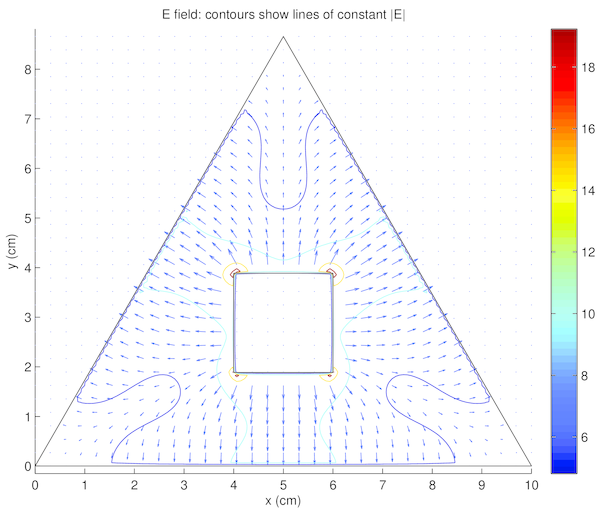
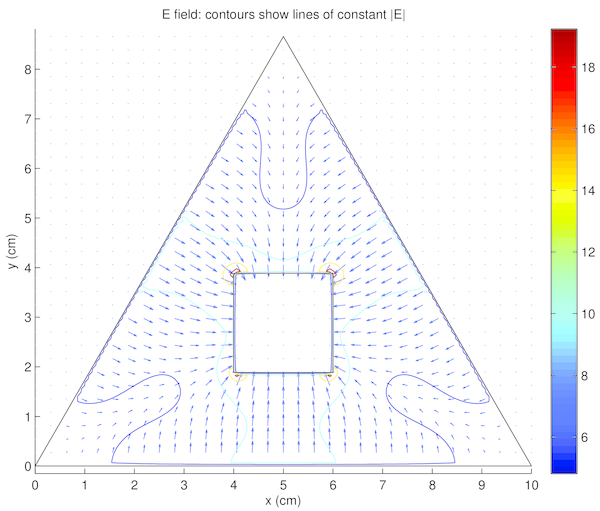
The electric field in tables 2, 3, 4, and 5 right) similarly demonstrated the expected properties. The field formed a smooth vector field, with no noticeable curl. The electric field also pointed from positive voltage to negative voltage, as expected. Finally, vectors intersected conductor surfaces at approximately 90. These properties were again expected [5], and supported confidence in the accuracy of the simulation.
Interestingly noted was that tables 2 and 4 were identical, with the exception of the colour scales in tables 2 and 4 left), as were tables 3 and 5. This phenomena is due to the voltage field being described by linear differential equations. Thus linearly translated boundary conditions yield correspondingly linearly scaled solutions. The electric field, however, is related by the derivative of the voltage field. Therefore, constant translations have no effect on the electric field, as demonstrated in tables 2 and 4 right), and tables 3 and 5 right). For the same reasons, the voltage fields in tables 2 and 4 left) were opposite to those in tables 3 and 5 left), and the electric fields in tables 2 and 4 right) were equal in magnitude (see the contour lines) and opposite in direction to those in tables 3 and 5 right). The boundary conditions between these two pairs were simply reversed.
Finally, table fig:v_convergence shows the calculated voltage for a given \(d_x\). Here it was noted that the variation between Voltage estimates was considerably lower for low values of \(d_x\) and increased with \(d_x\). This result was consistent with the theory outlined in equations \eqref{eq:1stO_FD_x}, \eqref{eq:1stO_FD_y}, \eqref{eq:2ndO_FD_x}, and \eqref{eq:2ndO_FD_y}, stating the associated error was in the order of the square of \(d_x\).
6 Conclusion
A numerical solution to the voltage and electrical field in a two-dimensional cross section of a coaxial cable, where the outer shield was an equilateral triangle with sides of 10 cm, and the core was a square with sides of 2 cm, was developed using methods. The accuracy of this method was verified using empirical means, based on qualitative observations of the resultant fields. These results indicated confidence in the accuracy of the method. Additional properties of the linearity of the electrical and voltage fields were noted, specifically the invariance of the electric field under boundary voltage translation, given the difference was the same.
7 Appendix: MATLAB Code
References
| [1] | E. W. Weisstein, “Laplace's equation. From MathWorld---A Wolfram Web Resource.” http://mathworld.wolfram.com/LaplacesEquation.html. Accessed: 11/4/2015. |
| [2] | J. D. Hoffman and S. Frankel, Numerical methods for engineers and scientists. CRC press, 2001. |
| [3] | D. Kosov, “EE4710 prac 2 description--Finite difference method for numerical solution to Laplace equation,” 2015. |
| [4] | D. Zill, W. S. Wright, and M. R. Cullen, Advanced engineering mathematics. Jones & Bartlett Learning, 2011. |
| [5] | D. J. Griffiths and R. College, Introduction to electrodynamics, vol. 3. Prentice Hall Upper Saddle River, NJ, 1999. |