Journal Club: Understanding deep learning requires rethinking generalization
Next Tuesday I will be leading IEEE-QLD’s 1st Tuesday Journal Paper Club, where we will be discussing the article Understanding deep learning requires rethinking generalization by Zhang, Bengio, Hardt, Recht and Vinyals, which was presented at ICLR2017. I selected this paper because it is often said that “we don’t even understand why deep learning works.” I believe this statement refers to two things, firstly the difficulty in explainability, tying in with the “right to explanation,” but secondly the higher level explanation of generalisation dealt with in this paper. I did not have as good a grasp of the latter, so this was a good opportunity to learn.
I have a good grasp on many of the concept in machine learning, however I am not actively involved in machine learning professionally, day-to-day. This presentation will also be aimed towards an audience of similar skill, and I hope to cover the some of the required topics along the way. With this in mind, I am sure I may miss some of the more nuanced take-aways from the paper.
The capacity of neural networks
In the first technical section, the authors introduce the main aspects of their methodology, which involves invoking various forms of randomisation on datasets. The dataset considered here is CIFAR10, which contains 60,000 samples split equally between 10 classes, airplane, automobile, bird, cat, deer, dog, frog, horse, ship, and truck.
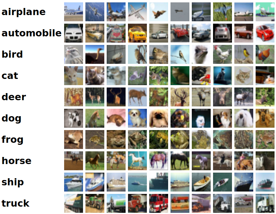
The preview for the CIFAR10 dataset.
The motivation is to create two datasets with identical statistical properties, one based on the real training set and one which has been randomised. This randomisation is achieved in five ways:
- by randomly reassigning each label,
- by randomly reassigning some labels, with probability (p),
- by randomly permuting pixels with the same permutation for all images, basically ruining shapes within the image,
- by randomly permuting pixels with different permutations for all images, ruining all spatial information but retaining the distribution,
- by randomly sampling each pixel from a distribution with the same mean and variance to the original data set.
Neural networks have been demonstrated many times to be able to generalise very well on CIFAR10. By creating a parallel dataset in which we randomise the labels, we can create a dataset with similar properties to which we will see a very low generalisation error.
Importantly, we should stop at this point, before conducting the test, to consider what we expect to happen.
- We aren’t too sure what the training error will be, as we intend to test the capacity of the networks. The higher the capacity, the lower the training error we should expect.
- For the uncorrupted labels, we expect a reasonably low test error and generalisation, consistent with previous experiments (e.g., competition results).
- For the corrupted labels, we expect test accuracy to be just 10% (i.e., random chance) and so the test error should be 90%.
- In training for the corrupted labels, we might expect to see some difficulty in training (much slower, or stopping and starting, for instance).
First, we will look at Figure 1 (b) and (c), as these results were relatively unsurprising. As we increase (p), the level of label corruption, the convergence slows down, and the test error steadily increases to 90%.
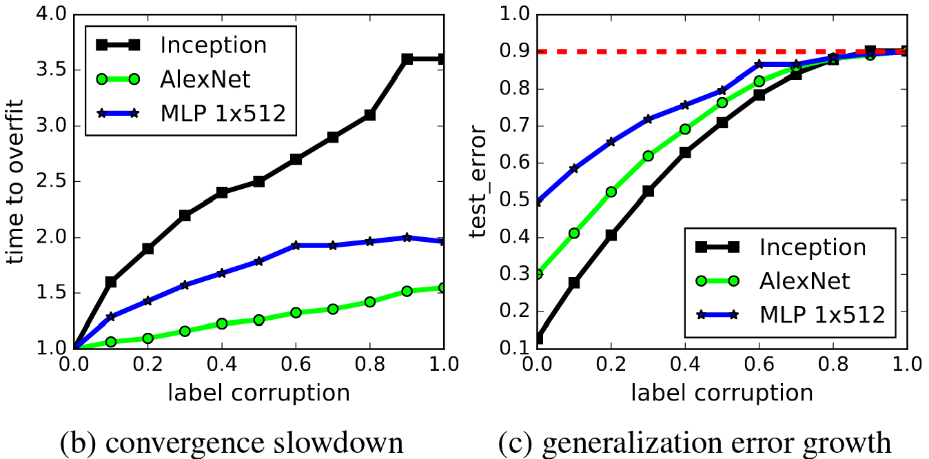
Figure 1 (b) and (c) from the paper.
Figure 1 (a) shows some potentially more interesting results. Firstly, all of the datasets can be completely learnt, indicating the networks have more than enough capacity for the training images. Potentially more interesting is that although the randomised datasets took longer to train, it appears the the gradient, or the learning rate, is quite similar for all datasets once the training “gets going”. It appears that once the initial large errors due to uncorrelated labels are overcome, the randomised problems are not even significantly harder!
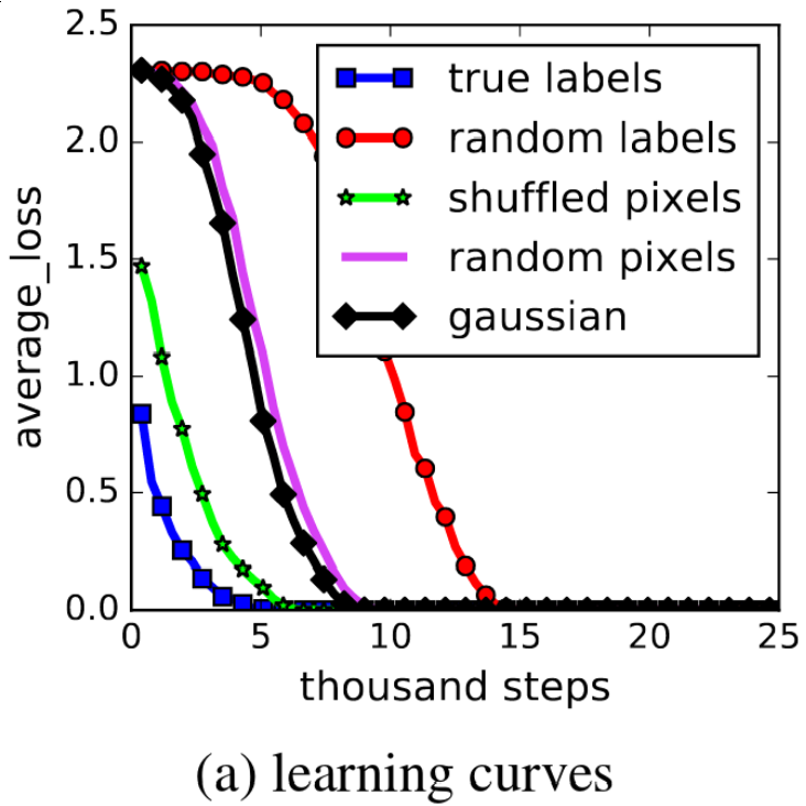
Figure 1 (a) from the paper.
Another interesting thing I found was the fact that random labels took the longest to train. Intuitively, I had expected the random pixels or Gaussian datasets to be harder. The authors have an intuitive explanation for this. Imagine you have a well separated dataset, as shown below in the top left plot, and you then shuffle the labels and have to draw a line separating the classes. Because the classes were clustered together quite closely originally, you have to be quite careful in drawing that line. Now imaging you have a dataset that is spread more uniformly and randomly over the space, which you also shuffle and draw a separating line. This line should, on average, be easier to draw, as the points should be more spread. In this way, we can understand that the similarities in images, which after shuffling have different labels, can actually make learning harder.
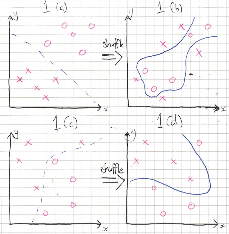
(a) Two clusters. (b) Two clusters after shuffling. (c) Randomly distributed labels. (d) Randomly distributed labels after shuffling.
This example also introduces the concept of shattering, which can be thought of as the ability to draw the separating line between the classes. In the top left plot, we could say that the data is shattered by a straight line, however the other plots require more complex lines to shatter the data. The concept of shattering is a little more rigorous than this, but this basic understanding will suffice.
The concept of shattering is required to understand the next concept, VC dimension. The VC dimension of a model is maximum number of points a model can always shatter for a given class of dataset. For example, shown below, we can see that for a dataset of 3 non-colinear points, a model of a straight line has VC dimension 3.
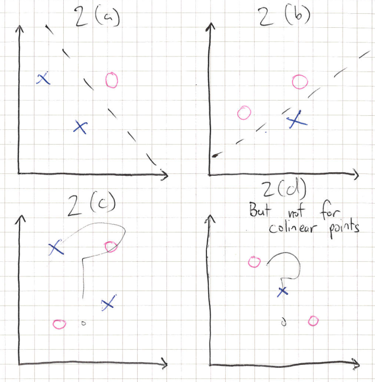
(a) and (b) We can see that we can shatter three points in two dimensions with a straight line. (c) We cannot necessarily shatter four points, so the VC dimension is 3. (d) VC dimension of 3 only applies to non-colinear points.
In terms of a linear model, imagine we have a linear relationship with some noise. If we try and fit a high-order polynomial, we know from experience that this may not generalise well, and will overfit. We can see this as using a model with too high of a complexity. We could see that potentially, measuring how much higher the complexity of the model vs. the underlying data may indicate or predict the generalisation error.
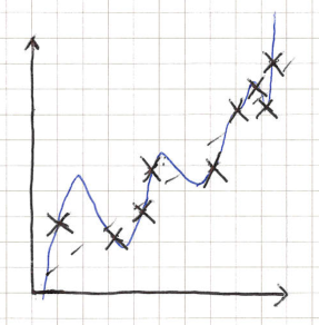
Excessive high complexity (i.e., VC dimension) may predict generalisation?
Now here comes the hand-waving part where I don’t completely understand what is happening. A complexity measure of a model, such as the VC dimension, or the Rademacher complexity, which I haven’t discussed, can be used to prove a bound exists on generalization error. Potentially, this could be used to explain why deep learning is able to generalise so well! A post by Mostafa Samir goes through a lot of the theory involved. But alas, the fact that we are able to completely memorise the dataset means that this is not a satisfactory explanation.
Other authors have tried to argue that the sensitivity of an algorithm may be able to explain generalisation bounds. The uniform stability of an algorithm is a measure of sensitivity of a trained model to missing a data point, and we would say an algorithm is stable if roughly the same model is generated. Intuitively, such a property could lead to a reduced generalisation error: imagine that we moved that missing data point to the test set, if it hadn’t changed the model significantly we might imagine it is likely to be classified correctly. However, the authors argue this property is a property only of the training algorithm, and so cannot explain why our experiment, which maintained the same algorithm, changing only the data, yielded such different generalisation properties.
The role of regularisation
The authors go on to investigate the effect of regularisation. Three types of regularisation were considered, data augmentation, weight decay and dropout.
Data augmentation consists of expanding the training data by adding modified versions of the dataset. These additional training data might be rotated, cropped, scaled or otherwise transformed versions of the data. My first thought was “why is this a regularisation technique?” User99889 on Cross Validated gives an intuitive explanation: we are attempting to enforce a prior, that we know that the augmentations we apply don’t change the classification. This makes sense only if you consider the data augmentation process to be a stage in the training algorithm, which I guess I had not previously.
Weight decay causes weights to exponentially decay each iteration, penalising large weights and forcing the network to “use it or lose it”. Large weights that may not be activated during training could cause large changes on unseen data during generalisation. In dropout, nodes are randomly masked out (i.e., give an output of 0) with some probability at each iteration. This forces redundancy in learnt responses.
In this experiment, the authors look at both the test and training accuracy with data augmentation and weight decay turned on and off. For the CIFAR10 dataset, greater than 99% training accuracy was achieved in all cases. We might have intuitively expected that regularisation limited the complexity or expressivity of the network, which might explain why regularisation can increase generalisation. However, these results show that we can still almost perfectly memorise the given dataset, giving maximum expressivity: so again the authors have shown that the complexity measure is not indicating generalisation.
Another result here shows that even without any explicit regularisation, very competitive generalisation results are yielded. Hence, the regularisation, or at least this explicit regularisation, is not the primary reason for the generalisation.
The authors also investigate implicit regularisation, showing that early stopping only has a potential impact where other regularisation is not used, and that batch normalisation does not explain the level of generalisation. They conclude that implicit (or explicit) regularisation helps generalisation, but does not fully explain it. I, however, disagree at this point. There are obviously infinitely many solutions that can perform well on these test sets, since they are able to be memorised. Some form of regularisation, obviously implicit, must explain why the given model which generalises was chosen, almost by the loose definition of regularisation.
Finite sample expressivity
In this section, the authors explain that often, the capacity of a network is measured by what class of functions it is able to express. They argue that, perhaps, a more useful insight is to derive what size network is required to fully express a given sample size. In the appendix, they show a proof that a two-layer network of size \(2n + d\) is sufficient to express \(n\) data points in \(d\) dimensions, and take steps to show bounds on the order required of the width if deeper networks are allowed. This seems a logical way to consider the capacity of a network, given the previous experiments.
Implicit regularisation: an appeal to linear models
The authors finish the article by analysing linear models. They show that for a linear model with enough dimension to have an infinite solutions (i.e., higher dimension than or equal to the number of test points), choosing a solutions that minimises the \(\ell_2\)-norm can have good generalisation properties. In fact, the the MNIST dataset, a handwritten digit dataset, they are able to achieve just 1.2% test error. They can reduce this further to 0.6% by pre-processing with Gabor wavelets, which provide features based on the structure of lines in the images. The authors then speculate that perhaps the \(\ell_2\)-norm of the solution may provide insight into the generalisation properties. But alas, the \(\ell_2\)-norm increased when Gabor wavelets were used, showing that even for linear models we don’t have a good way to predict or bound generalisation error.
Summary
I thought this was an interesting, high level paper. For the journal club I am presenting, where most attendees are familiar with nerual networks and deep learning, but not intimately, I am hoping explaining the concepts in this paper will provide a good introduction, with some novel content, without diving too deep into the technical.